使用Java代码实现傅里叶变换_java傅立叶变黑白-程序员宅基地
说明
-
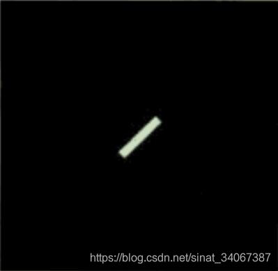
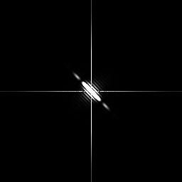
该代码源自java使用傅里叶变换,对其进行了部分优化,可以实现将灰度图像转换为频率域图像,以及从频率域恢复为原图像。
-
初次接触傅里叶算法,有很多新概念,理解起来比较困难,需要多看几遍,参考链接都在文章最后。
-
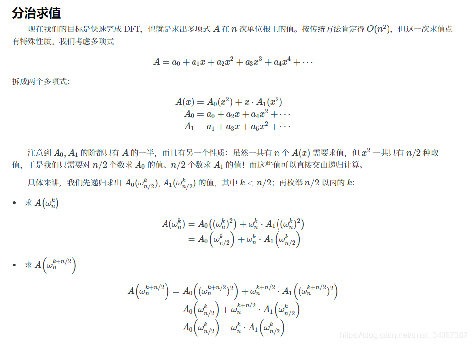
这边的代码逻辑其实很简单,就是输入一组复数数组,进行处理后,返回相同长度的复数数组,处理的算法和下面的公式有关,然后和三角函数没有太大关联,但想理清整个傅里叶变换,三角函数还是绕不过去的。
-
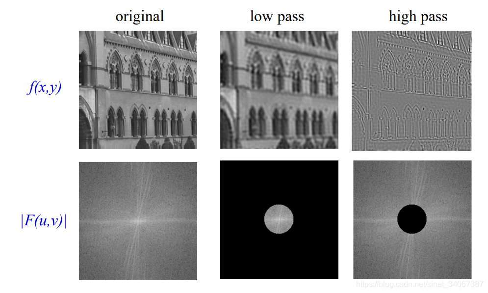
通过去除图像中的低频率来提取边缘,或者通过去除高频率来模糊图像已经实现了,在recover()方法里面,去除高频率需要手动去除注释。
代码
主类
package com.example.springboot01.util;

import org.junit.Test;

import javax.imageio.ImageIO;
import java.awt.image.BufferedImage;
import java.io.File;
import java.io.IOException;

/**
 * 代码参考:https://blog.csdn.net/wangjichen_1/article/details/51120194
 */
public class FourierTransformer {


	@Test
	public void test() throws IOException {

		String fromPic = "C:\\Users\\Dell\\Pictures\\aaa.jpg";
		BufferedImage bufferedImage = ImageIO.read(new File(fromPic));

		// 转换为频率域图像
		BufferedImage destImg = convert(bufferedImage);
		// 从频率域恢复为原图片,未实现去除高频率功能
		// BufferedImage destImg = recover(bufferedImage);
		File newFile = new File("d:\\test10.jpg");
		ImageIO.write(destImg, "jpg", newFile);
	}

	/**
	 * 生成频率域图像
	 * @param srcImage
	 * @return
	 */
	public BufferedImage convert(BufferedImage srcImage) {

		int iw = srcImage.getWidth();
		int ih = srcImage.getHeight();
		int[] pixels = new int[iw * ih];
		int[] newPixels;
		srcImage.getRGB(0, 0, iw, ih, pixels, 0, iw);

		// 赋初值
		int w = 1;
		int h = 1;
		// 计算进行付立叶变换的宽度和高度(2的整数次方)
		while (w * 2 <= iw) {

			w *= 2;
		}
		while (h * 2 <= ih) {

			h *= 2;
		}
		// 分配内存
		// 从左往右,从上往下排序
		Complex[] src = new Complex[h * w];
		// 从左往右,从上往下排序
		Complex[] dest = new Complex[h * w];
		newPixels = new int[h * w];

		for (int i = 0; i < h; i++) {

			for (int j = 0; j < w; j++) {

				// 初始化src,dest
				dest[i * w + j] = new Complex();
				// 获取蓝色通道分量,也就是像素点的灰度值
				src[i * w + j] = new Complex(pixels[i * iw + j] & 0xff, 0);
			}
		}

		// 在y方向上进行快速傅立叶变换
		//
		// 一行一行的处理
		// 处理完后第一列都是各自行里面的最大值
		//
		for (int i = 0; i < h; i++) {

			Complex[] temp = new Complex[w];
			for (int k = 0; k < w; k++) {

				temp[k] = src[i * w + k];
			}
			temp = FFT.fft(temp);

			for (int k = 0; k < w; k++) {

				dest[i * w + k] = temp[k];
			}
		}

		// 对x方向进行傅立叶变换
		// 一列一列的处理,从左往右
		// 处理完后第一行都是各自列里面的最大值
		for (int i = 0; i < w; i++) {

			Complex[] temp = new Complex[h];
			for (int k = 0; k < h; k++) {

				temp[k] = dest[k * w + i];
			}
			temp = FFT.fft(temp);

			for (int k = 0; k < h; k++) {

				dest[k * w + i] = temp[k];
			}
		}

		// 打印傅里叶频率域图像
		for (int i = 0; i < h; i++) {

			for (int j = 0; j < w; j++) {

				// 从左到右,从上到下遍历
				double re = dest[i * w + j].re;
				double im = dest[i * w + j].im;

				int ii = 0, jj = 0;
				// 缩小数值,方便展示
				int temp = (int) (Math.sqrt(re * re + im * im) / 100);

				// 用十字将图像切割为4等分,然后每个部分旋转180度,再拼接起来,方便观察
				if (i < h / 2) {

					ii = i + h / 2;
				} else {

					ii = i - h / 2;
				}
				if (j < w / 2) {

					jj = j + w / 2;
				} else {

					jj = j - w / 2;
				}
				newPixels[ii * w + jj] = (clamp(temp) << 16) | (clamp(temp) << 8) | clamp(temp);;
			}
		}

		BufferedImage destImg = new BufferedImage(w, h, BufferedImage.TYPE_BYTE_GRAY);
		destImg.setRGB(0, 0, w, h, newPixels, 0, w);

		return destImg;
	}

	/**
	 * 从频率还原为图像
	 * 已经实现了通过去除低频率提取边缘和通过去除高频率模糊图像两个功能
	 * @param srcImage
	 * @return
	 */
	public BufferedImage recover(BufferedImage srcImage) {

		int iw = srcImage.getWidth();
		int ih = srcImage.getHeight();
		int[] pixels = new int[iw * ih];
		int[] newPixels;
		srcImage.getRGB(0, 0, iw, ih, pixels, 0, iw);

		// 赋初值
		int w = 1;
		int h = 1;
		// 计算进行付立叶变换的宽度和高度(2的整数次方)
		while (w * 2 <= iw) {

			w *= 2;
		}
		while (h * 2 <= ih) {

			h *= 2;
		}
		// 分配内存
		// 从左往右,从上往下排序
		Complex[] src = new Complex[h * w];
		// 从左往右,从上往下排序
		Complex[] dest = new Complex[h * w];
		newPixels = new int[h * w];

		for (int i = 0; i < h; i++) {

			for (int j = 0; j < w; j++) {

				// 初始化src,dest
				dest[i * w + j] = new Complex();
				// 获取蓝色通道分量,也就是像素点的灰度值
				src[i * w + j] = new Complex(pixels[i * iw + j] & 0xff, 0);
			}
		}

		// 在y方向上进行快速傅立叶变换
		//
		// 先一行一行的处理
		// 处理完后第一列都是各自行里面的最大值
		//
		for (int i = 0; i < h; i++) {

			Complex[] temp = new Complex[w];
			for (int k = 0; k < w; k++) {

				temp[k] = src[i * w + k];
			}
			temp = FFT.fft(temp);

			for (int k = 0; k < w; k++) {

				dest[i * w + k] = temp[k];
			}
		}

		// 对x方向进行傅立叶变换
		// 再一列一列的处理,从左往右
		// 处理完后第一行都是各自列里面的最大值
		for (int i = 0; i < w; i++) {

			Complex[] temp = new Complex[h];
			for (int k = 0; k < h; k++) {

				temp[k] = dest[k * w + i];
			}
			temp = FFT.fft(temp);

			for (int k = 0; k < h; k++) {

				dest[k * w + i] = temp[k];
			}
		}

		// 去除指定频率部分,然后还原为图像
		int halfWidth = w/2;
		int halfHeight = h/2;
		// 比例越小,边界越突出
		double res = 0.24;

		// 比例越大,图片越模糊
		double del = 0.93;
		// 先对列进行逆傅里叶变换,并去除指定频率。和傅里叶变换顺序相反
		for (int i = 0; i < w; i++) {

			Complex[] temp = new Complex[h];
			for (int k = 0; k < h; k++) {

				// 去除低频率,保留边缘,因为频率图尚未做十字切割并分别旋转180度,所以此时图像dest[] 的四个角落是低频率,而中心部分是高频率
				// 第一个点(0,0)不能删除,删掉后整张图片就变黑了
				if (i == 0 && k == 0) {

					temp[k] = dest[k * w + i];
				} else if ((i <res*halfWidth && k < res*halfHeight) || (i <res*halfWidth && k > (1-res)*halfHeight)
						|| (i > (1-res)*halfWidth && k <res*halfHeight) || (i > (1-res)*halfWidth && k > (1-res)*halfHeight)) {

					temp[k] = new Complex(0, 0);
				} else {

					temp[k] = dest[k * w + i];
				}

				// 去除高频率,模糊图像。和去除低频率代码冲突,需要先屏蔽上面去除低频率的代码才能执行
				/*if ((i > ((1-del)*halfWidth) && k > ((1-del)*halfHeight)) && (i <((1+del)*halfWidth) && k < ((1+del)*halfHeight))) {
					temp[k] = new Complex(0, 0);
				} else {
					temp[k] = dest[k * w + i];
				}*/
			}
			temp = FFT.ifft(temp);
			for (int k = 0; k < h; k++) {

				// 这边需要除以N,也就是temp[]的长度
				dest[k * w + i].im = temp[k].im / h;
				dest[k * w + i].re = temp[k].re / h;
			}
		}

		// 再对行进行逆傅里叶变换
        for (int i = 0; i < h; i++) {

            Complex[] temp = new Complex[w];
            for (int k = 0; k < w; k++) {

            	temp[k] = dest[i * w + k];
            }
            temp = FFT.ifft(temp);
            for (int k = 0; k < w; k++) {

            	// 这边需要除以N,也就是temp[]的长度
				dest[i * w + k].im = temp[k].im / w;
                dest[i * w + k].re = temp[k].re / w;
            }
        }

        for (int i = 0; i < h; i++) {

            for (int j = 0; j < w; j++) {

                // 从左到右,从上到下遍历
                double re = dest[i * w + j].re;
                int temp = (int) re;
                newPixels[i * w + j] = (clamp(temp) << 16) | (clamp(temp) << 8) | clamp(temp);;
            }
        }

        BufferedImage destImg = new BufferedImage(w, h, BufferedImage.TYPE_BYTE_GRAY);
        destImg.setRGB(0, 0, w, h, newPixels, 0, w);

        return destImg;
	}

	/**
	 * 如果像素点的值超过了0-255的范围,予以调整
	 *
	 * @param value 输入值
	 * @return 输出值
	 */
	private int clamp(int value) {

		return value > 255 ? 255 : (Math.max(value, 0));
	}
}
傅里叶变换类
package com.example.springboot01.util;

/**
 * 快速傅里叶变换
 * 傅里叶介绍参考:https://www.ruanx.net/fft/
 *	https://blog.csdn.net/YY_Tina/article/details/88361459
 */
public class FFT {


	/**
	 * 快速傅里叶变换
	 * @param x
	 * @return
	 */
	// compute the FFT of x[], assuming its length is a power of 2
	public static Complex[] fft(Complex[] x) {

		int N = x.length;

		// base case
		if (N == 1)
			return new Complex[] {
     x[0] };

		// radix 2 Cooley-Tukey FFT
		if (N % 2 != 0) {

			throw new RuntimeException("N is not a power of 2");
		}

		// fft of even terms
		Complex[] even = new Complex[N / 2];
		for (int k = 0; k < N / 2; k++) {

			even[k] = x[2 * k];
		}
		Complex[] q = fft(even);

		// fft of odd terms
		Complex[] odd = even; // reuse the array
		for (int k = 0; k < N / 2; k++) {

			odd[k] = x[2 * k + 1];
		}
		Complex[] r = fft(odd);

		// combine
		Complex[] y = new Complex[N];
		for (int k = 0; k < N / 2; k++) {

			double kth = 2 * k * Math.PI / N;
			Complex wk = new Complex(Math.cos(kth), Math.sin(kth));
			y[k] = q[k].plus(wk.times(r[k]));
			y[k + N / 2] = q[k].minus(wk.times(r[k]));
		}
		return y;
	}


	/**
	 * 逆快速傅里叶变换
	 * 与fft()相比,只修改了kth的值
	 * @param x
	 */
	public static Complex[] ifft(Complex[] x) {

		int N = x.length;

		// base case
		if (N == 1)
			return new Complex[] {
     x[0] };

		// radix 2 Cooley-Tukey FFT
		if (N % 2 != 0) {

			throw new RuntimeException("N is not a power of 2");
		}

		// fft of even terms
		Complex[] even = new Complex[N / 2];
		for (int k = 0; k < N / 2; k++) {

			even[k] = x[2 * k];
		}
		Complex[] q = ifft(even);

		// fft of odd terms
		Complex[] odd = even; // reuse the array
		for (int k = 0; k < N / 2; k++) {

			odd[k] = x[2 * k + 1];
		}
		Complex[] r = ifft(odd);

		// combine
		Complex[] y = new Complex[N];
		for (int k = 0; k < N / 2; k++) {

			// 这边有区别
			double kth = 2 * (N - k) * Math.PI / N;
			Complex wk = new Complex(Math.cos(kth), Math.sin(kth));
			y[k] = q[k].plus(wk.times(r[k]));
			y[k + N / 2] = q[k].minus(wk.times(r[k]));
		}
		return y;
	}


}
复数类
package com.example.springboot01.util;

/**
 * 复数类
 */
public class Complex {

    public  double re;   // the real part
    public  double im;   // the imaginary part

    public Complex() {

        re = 0;
        im = 0;
    }

    // create a new object with the given real and imaginary parts
    public Complex(double real, double imag) {

        re = real;
        im = imag;
    }

    // return a string representation of the invoking Complex object
    public String toString() {

        if (im == 0) return re + "";
        if (re == 0) return im + "i";
        if (im <  0) return re + " - " + (-im) + "i";
        return re + " + " + im + "i";
    }

    // return abs/modulus/magnitude and angle/phase/argument
    public double abs()   {
     return Math.hypot(re, im); }  // Math.sqrt(re*re + im*im)
    public double phase() {
     return Math.atan2(im, re); }  // between -pi and pi

    // return a new Complex object whose value is (this + b)
    public Complex plus(Complex b) {

        Complex a = this;             // invoking object
        double real = a.re + b.re;
        double imag = a.im + b.im;
        return new Complex(real, imag);
    }

    // return a new Complex object whose value is (this - b)
    public Complex minus(Complex b) {

        Complex a = this;
        double real = a.re - b.re;
        double imag = a.im - b.im;
        return new Complex(real, imag);
    }

    // return a new Complex object whose value is (this * b)
    public Complex times(Complex b) {

        Complex a = this;
        double real = a.re * b.re - a.im * b.im;
        double imag = a.re * b.im + a.im * b.re;
        return new Complex(real, imag);
    }

    // scalar multiplication
    // return a new object whose value is (this * alpha)
    public Complex times(double alpha) {

        return new Complex(alpha * re, alpha * im);
    }

    // return a new Complex object whose value is the conjugate of this
    public Complex conjugate() {
      return new Complex(re, -im); }

    // return a new Complex object whose value is the reciprocal of this
    public Complex reciprocal() {

        double scale = re*re + im*im;
        return new Complex(re / scale, -im / scale);
    }

    // return the real or imaginary part
    public double re() {
     return re; }
    public double im() {
     return im; }

    // return a / b
    public Complex divides(Complex b) {

        Complex a = this;
        return a.times(b.reciprocal());
    }

    // return a new Complex object whose value is the complex exponential of this
    public Complex exp() {

        return new Complex(Math.exp(re) * Math.cos(im), Math.exp(re) * Math.sin(im));
    }

    // return a new Complex object whose value is the complex sine of this
    public Complex sin() {

        return new Complex(Math.sin(re) * Math.cosh(im), Math.cos(re) * Math.sinh(im));
    }

    // return a new Complex object whose value is the complex cosine of this
    public Complex cos() {

        return new Complex(Math.cos(re) * Math.cosh(im), -Math.sin(re) * Math.sinh(im));
    }

    // return a new Complex object whose value is the complex tangent of this
    public Complex tan() {

        return sin().divides(cos());
    }


    // a static version of plus
    public static Complex plus(Complex a, Complex b) {

        double real = a.re + b.re;
        double imag = a.im + b.im;
        Complex sum = new Complex(real, imag);
        return sum;
    }
}
效果图
参考
java使用傅里叶变换,得到变换之后的傅里叶频谱图像。
快速傅里叶变换
快速傅里叶变换(FFT)和逆快速傅里叶变换(IFFT)
傅里叶分析之掐死教程(完整版)
图像傅里叶变换
二维傅里叶变换深度研究-图像与其频域关系
傅里叶变换在工程中的一些应用
形象理解二维傅里叶变换
智能推荐
分布式光纤传感器的全球与中国市场2022-2028年:技术、参与者、趋势、市场规模及占有率研究报告_预计2026年中国分布式传感器市场规模有多大-程序员宅基地
文章浏览阅读3.2k次。本文研究全球与中国市场分布式光纤传感器的发展现状及未来发展趋势,分别从生产和消费的角度分析分布式光纤传感器的主要生产地区、主要消费地区以及主要的生产商。重点分析全球与中国市场的主要厂商产品特点、产品规格、不同规格产品的价格、产量、产值及全球和中国市场主要生产商的市场份额。主要生产商包括:FISO TechnologiesBrugg KabelSensor HighwayOmnisensAFL GlobalQinetiQ GroupLockheed MartinOSENSA Innovati_预计2026年中国分布式传感器市场规模有多大
07_08 常用组合逻辑电路结构——为IC设计的延时估计铺垫_基4布斯算法代码-程序员宅基地
文章浏览阅读1.1k次,点赞2次,收藏12次。常用组合逻辑电路结构——为IC设计的延时估计铺垫学习目的:估计模块间的delay,确保写的代码的timing 综合能给到多少HZ,以满足需求!_基4布斯算法代码
OpenAI Manager助手(基于SpringBoot和Vue)_chatgpt网页版-程序员宅基地
文章浏览阅读3.3k次,点赞3次,收藏5次。OpenAI Manager助手(基于SpringBoot和Vue)_chatgpt网页版
关于美国计算机奥赛USACO,你想知道的都在这_usaco可以多次提交吗-程序员宅基地
文章浏览阅读2.2k次。USACO自1992年举办,到目前为止已经举办了27届,目的是为了帮助美国信息学国家队选拔IOI的队员,目前逐渐发展为全球热门的线上赛事,成为美国大学申请条件下,含金量相当高的官方竞赛。USACO的比赛成绩可以助力计算机专业留学,越来越多的学生进入了康奈尔,麻省理工,普林斯顿,哈佛和耶鲁等大学,这些同学的共同点是他们都参加了美国计算机科学竞赛(USACO),并且取得过非常好的成绩。适合参赛人群USACO适合国内在读学生有意向申请美国大学的或者想锻炼自己编程能力的同学,高三学生也可以参加12月的第_usaco可以多次提交吗
MySQL存储过程和自定义函数_mysql自定义函数和存储过程-程序员宅基地
文章浏览阅读394次。1.1 存储程序1.2 创建存储过程1.3 创建自定义函数1.3.1 示例1.4 自定义函数和存储过程的区别1.5 变量的使用1.6 定义条件和处理程序1.6.1 定义条件1.6.1.1 示例1.6.2 定义处理程序1.6.2.1 示例1.7 光标的使用1.7.1 声明光标1.7.2 打开光标1.7.3 使用光标1.7.4 关闭光标1.8 流程控制的使用1.8.1 IF语句1.8.2 CASE语句1.8.3 LOOP语句1.8.4 LEAVE语句1.8.5 ITERATE语句1.8.6 REPEAT语句。_mysql自定义函数和存储过程
半导体基础知识与PN结_本征半导体电流为0-程序员宅基地
文章浏览阅读188次。半导体二极管——集成电路最小组成单元。_本征半导体电流为0
随便推点
【Unity3d Shader】水面和岩浆效果_unity 岩浆shader-程序员宅基地
文章浏览阅读2.8k次,点赞3次,收藏18次。游戏水面特效实现方式太多。咱们这边介绍的是一最简单的UV动画(无顶点位移),整个mesh由4个顶点构成。实现了水面效果(左图),不动代码稍微修改下参数和贴图可以实现岩浆效果(右图)。有要思路是1,uv按时间去做正弦波移动2,在1的基础上加个凹凸图混合uv3,在1、2的基础上加个水流方向4,加上对雾效的支持,如没必要请自行删除雾效代码(把包含fog的几行代码删除)S..._unity 岩浆shader
广义线性模型——Logistic回归模型(1)_广义线性回归模型-程序员宅基地
文章浏览阅读5k次。广义线性模型是线性模型的扩展,它通过连接函数建立响应变量的数学期望值与线性组合的预测变量之间的关系。广义线性模型拟合的形式为:其中g(μY)是条件均值的函数(称为连接函数)。另外,你可放松Y为正态分布的假设,改为Y 服从指数分布族中的一种分布即可。设定好连接函数和概率分布后,便可以通过最大似然估计的多次迭代推导出各参数值。在大部分情况下,线性模型就可以通过一系列连续型或类别型预测变量来预测正态分布的响应变量的工作。但是,有时候我们要进行非正态因变量的分析,例如:(1)类别型.._广义线性回归模型
HTML+CSS大作业 环境网页设计与实现(垃圾分类) web前端开发技术 web课程设计 网页规划与设计_垃圾分类网页设计目标怎么写-程序员宅基地
文章浏览阅读69次。环境保护、 保护地球、 校园环保、垃圾分类、绿色家园、等网站的设计与制作。 总结了一些学生网页制作的经验:一般的网页需要融入以下知识点:div+css布局、浮动、定位、高级css、表格、表单及验证、js轮播图、音频 视频 Flash的应用、ul li、下拉导航栏、鼠标划过效果等知识点,网页的风格主题也很全面:如爱好、风景、校园、美食、动漫、游戏、咖啡、音乐、家乡、电影、名人、商城以及个人主页等主题,学生、新手可参考下方页面的布局和设计和HTML源码(有用点赞△) 一套A+的网_垃圾分类网页设计目标怎么写
C# .Net 发布后,把dll全部放在一个文件夹中,让软件目录更整洁_.net dll 全局目录-程序员宅基地
文章浏览阅读614次,点赞7次,收藏11次。之前找到一个修改 exe 中 DLL地址 的方法, 不太好使,虽然能正确启动, 但无法改变 exe 的工作目录,这就影响了.Net 中很多获取 exe 执行目录来拼接的地址 ( 相对路径 ),比如 wwwroot 和 代码中相对目录还有一些复制到目录的普通文件 等等,它们的地址都会指向原来 exe 的目录, 而不是自定义的 “lib” 目录,根本原因就是没有修改 exe 的工作目录这次来搞一个启动程序,把 .net 的所有东西都放在一个文件夹,在文件夹同级的目录制作一个 exe._.net dll 全局目录
BRIEF特征点描述算法_breif description calculation 特征点-程序员宅基地
文章浏览阅读1.5k次。本文为转载,原博客地址:http://blog.csdn.net/hujingshuang/article/details/46910259简介 BRIEF是2010年的一篇名为《BRIEF:Binary Robust Independent Elementary Features》的文章中提出,BRIEF是对已检测到的特征点进行描述,它是一种二进制编码的描述子,摈弃了利用区域灰度..._breif description calculation 特征点
房屋租赁管理系统的设计和实现,SpringBoot计算机毕业设计论文_基于spring boot的房屋租赁系统论文-程序员宅基地
文章浏览阅读4.1k次,点赞21次,收藏79次。本文是《基于SpringBoot的房屋租赁管理系统》的配套原创说明文档,可以给应届毕业生提供格式撰写参考,也可以给开发类似系统的朋友们提供功能业务设计思路。_基于spring boot的房屋租赁系统论文