图像分割是将一幅图像分割成有意义区域的过程。区域可以是图像的前景与背景或 图像中一些单独的对象。这些区域可以利用一些诸如颜色、边界或近邻相似性等特 征进行构建。本章中，我们将看到一些不同的分割技术。

1、图割

（1）从图像创建图割

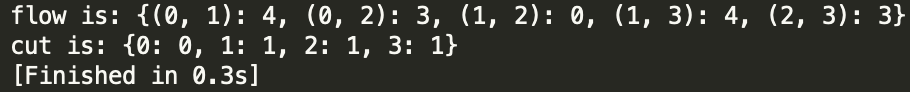
用 python-graph 工具包计算一幅较小的图 1 的最大流 / 最小割的简单例子:：

代码实现：

from pygraph.classes.digraph import digraph
from pygraph.algorithms.minmax import maximum_flow
gr = digraph()
gr.add_nodes([0,1,2,3])
gr.add_edge((0,1), wt=4)
gr.add_edge((1,2), wt=3)
gr.add_edge((2,3), wt=5)
gr.add_edge((0,2), wt=3)
gr.add_edge((1,3), wt=4)
flows,cuts = maximum_flow(gr, 0, 3)
print('flow is:' , flows)
print('cut is:' , cuts)

运行结果：

 

利用贝叶斯概率模型进行图割分割：

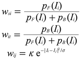
权重模型：像素 i 与像素 j 之间的边 的权重记为 wij，源点到像素 i 的权重记为 wsi，像素 i 到汇点的权重记为 wit。前景和背景计算概率 pF(Ii) 和 pB(Ii)，wij 描述了近邻间像素的相似性，相似像素权重趋近于 κ，不相 似的趋近于 0。参数 σ 表征了随着不相似性的增加，指数次幂衰减到 0 的快慢。公式如下：

代码实现：

# from scipy.misc import imresize  ##已被弃用，用from PIL import Image替代
import graphcut
from PIL import Image
from pylab import *

# 添加中文字体支持
from matplotlib.font_manager import FontProperties
font = FontProperties(fname=r"/System/Library/Fonts/PingFang.ttc", size=14)

# 读入图像
im = array(Image.open("../data/empire.jpg"))
h,w = im.shape[:2]
print(h,w)
scale = 0.05  #  scale = 0.265 ，scale*scale ~= 0.07跑起来非常慢,scale=0.05代码跑通比较快
num_px = int(w * scale)
num_py = int(h * scale) 
# imresize(im, 0.07,interp='bilinear')  ##imresize被scipy.misc弃用，用PIL库中的resize替代
im = array(Image.fromarray(im).resize((num_px,num_py),Image.BILINEAR))
size = im.shape[:2]
print(size)
rm = im

# 添加两个矩形训练区 
labels = np.zeros(size)
labels[3:18, 3:18] = -1
labels[-18:-3, -18:-3] = 1
# print(labels.size)
print("labels finish")

# 创建训练图
g = graphcut.build_bayes_graph(im, labels, kappa=1)
print("build_bayes_graph finish")

# 得到分割图
res = graphcut.cut_graph(g, size)
print("cut_graph finish")

#显示标记图
fig = figure()
subplot(131)
graphcut.show_labeling(im, labels)
gray()
title(u'标记图', fontproperties=font)
axis('off')

# #显示训练图
subplot(132)
imshow(rm) 
contour(labels,[-0.5,0.5],colors='blue') 
contour(labels,[0.5,1],colors='yellow') 
# gray()
title(u'训练图', fontproperties=font)
axis('off')

#显示分割图
subplot(133)
imshow(res)
gray()
title(u'分割图', fontproperties=font)
axis('off')
show()

# 保存figure中的灰度图像和积分图像
fig.savefig("../images/ch09/ch10_P215_Fig-2_bayes-cutgraph.jpg")

print("finish")

graphcut.py代码：

from pygraph.classes.digraph import digraph
from pygraph.algorithms.minmax import maximum_flow
import bayes
# import numpy as np
# import matplotlib.pyplot as plt
from pylab import *

def build_bayes_graph(im,labels,sigma=1e2,kappa=2):
### """从像素四邻域建立一个图，前景和背景(前景用 1 标记，背景用 -1 标记，
### 其他的用 0 标记)由 labels 决定，并用朴素贝叶斯分类器建模 """ 

	m,n = im.shape[:2]

	# 每行是一个像素的 RGB 向量 
	vim = im.reshape((-1,3))

	# 前景和背景(RGB)
	foreground = im[labels==1].reshape((-1,3)) 
	background = im[labels==-1].reshape((-1,3)) 
	train_data = [foreground,background]

	# 训练朴素贝叶斯分类器
	bc = bayes.BayesClassifier() 
	bc.train(train_data)

	# 获取所有像素的概率 
	bc_lables,prob = bc.classify(vim) 
	prob_fg = prob[0]
	prob_bg = prob[1]

	# 用m*n+2 个节点创建图
	gr = digraph() 
	gr.add_nodes(range(m*n+2))
	source = m*n # 倒数第二个是源点 
	sink = m*n+1 # 最后一个节点是汇点

	# 归一化
	for i in range(vim.shape[0]):
		vim[i] = vim[i] / linalg.norm(vim[i])

	# 遍历所有的节点，并添加边 
	for i in range(m*n):
		# 从源点添加边
		gr.add_edge((source,i), wt=(prob_fg[i]/(prob_fg[i]+prob_bg[i])))
		# 向汇点添加边
		gr.add_edge((i,sink), wt=(prob_bg[i]/(prob_fg[i]+prob_bg[i])))

	# 向相邻节点添加边
	if i%n != 0: #左边存在
		edge_wt = kappa*np.exp(-1.0*np.sum((vim[i]-vim[i-1])**2)/sigma)
		gr.add_edge((i,i-1), wt=edge_wt) 
	if (i+1)%n != 0: # 如果右边存在
		edge_wt = kappa*np.exp(-1.0*np.sum((vim[i]-vim[i+1])**2)/sigma)
		gr.add_edge((i,i+1), wt=edge_wt) 
	if i//n != 0: #如果上方存在
		edge_wt = kappa*np.exp(-1.0*np.sum((vim[i]-vim[i-n])**2)/sigma)
		gr.add_edge((i,i-n), wt=edge_wt) 
	if i//n != m-1: # 如果下方存在
		edge_wt = kappa*np.exp(-1.0*np.sum((vim[i]-vim[i+n])**2)/sigma) 
		gr.add_edge((i,i+n), wt=edge_wt)

	return gr

def show_labeling(im,labels):
	###""" 显示图像的前景和背景区域。前景 labels=1, 背景 labels=-1，其他 labels = 0 """
	imshow(im)
	contour(labels,[-0.5,0.5]) 
	contourf(labels,[-1,-0.5],colors='b',alpha=0.25) 
	contourf(labels,[0.5,1],colors='r',alpha=0.25) 
	axis('off')

def cut_graph(gr,imsize):
	###""" 用最大流对图 gr 进行分割，并返回分割结果的二值标记 """
	m,n = imsize
	source = m*n # 倒数第二个节点是源点 
	sink = m*n+1 # 倒数第一个是汇点

	# 对图进行分割
	flows,cuts = maximum_flow(gr,source,sink)

	# 将图转为带有标记的图像
	res = zeros(m*n)
	for pos,label in list(cuts.items())[:-2]: # 不要添加源点 / 汇点
		res[pos] = label

	return res.reshape((m,n))

按照原书中图像缩放为原图的0.07，宽高缩放因子scale = 0.265；这样程序跑起来太慢，所以将宽高缩放因子设为scale = 0.05，这样可以尽快验证程序逻辑是否正确。scale = 0.05时，标记图、训练图和分割图运行结果：

（2）用户交互式分割

代码实现：

# from scipy.misc import imresize
# from PCV.tools import graphcut
import graphcut
from PIL import Image
from pylab import *
# import numpy as np
# # import pylab as pl
# import matplotlib.pyplot as plt


# 添加中文字体支持
from matplotlib.font_manager import FontProperties
font = FontProperties(fname=r"/System/Library/Fonts/PingFang.ttc", size=14)

def create_msr_labels(m, lasso=False):
    """ Create label matrix for training from
    user annotations. """
    # rim = im.reshape((-1,2))
    # m = m.convert("L")
    size = m.shape[:2]
    # m = Image.fromarray(m.astype('uint8')).convert("L")
    # size = m.shape[:2]
    labels = zeros(size)
    # background
    labels[m == 0] = -1
    labels[m == 64] = -1
    # foreground
    if lasso:
        labels[m == 255] = 1
    else:
        labels[m == 128] = 1
    return labels

# load image and annotation map
im = array(Image.open('../data/book_perspective.JPG'))
m = array(Image.open('../data/book_perspective.bmp').convert('L'))

# resize
# scale = 0.32
scale = 0.05 #  scale = 0.32 ，scale*scale ~= 0.1跑起来非常慢,scale=0.05代码跑通比较快
# im = imresize(im, scale, interp='bilinear')
# m = imresize(m, scale, interp='nearest')
h1,w1 = im.shape[:2]
h2,w2 = m.shape[:2]
print(h1,w1)
print(h2,w2)
# num_px = int(h * np.sqrt(0.07))
# num_py = int(w * np.sqrt(0.07))
px1 = int(w1 * scale)
py1 = int(h1 * scale) 
px2 = int(w2 * scale)
py2 = int(h2 * scale)
# imresize(im, 0.07,interp='bilinear')  ##imresize被scipy.misc弃用，用PIL库中的resize替代
im = array(Image.fromarray(im).resize((px1,py1),Image.BILINEAR))
m = array(Image.fromarray(m).resize((px2,py2),Image.NEAREST))
oim = im
print(im.shape[:2])
print(m.shape[:2])
# create training labels
labels = create_msr_labels(m, False)
print('labels finish')
# build graph using annotations
g = graphcut.build_bayes_graph(im, labels, kappa=2)
print('build_bayes_graph finish')
# cut graph
res = graphcut.cut_graph(g, im.shape[:2])
print('cut_graph finish')
# remove parts in background
res[m == 0] = 1
res[m == 64] = 1
# labels[m == 0] = 1
# labels[m == 64] = 1

# plot original image 
fig = figure()
subplot(121)
imshow(im)
gray()
title(u'原始图', fontproperties=font)
axis('off')

#plot the result
subplot(122)
imshow(res)
gray()
xticks([])
yticks([])
title(u'分割图', fontproperties=font)
axis('off')

show()
fig.savefig('../images/ch09/labelplot.pdf')

print('finish')

按照原书中图像缩放为原图的0.1，宽高缩放因子scale = 0.32；这样程序跑起来太慢，所以将宽高缩放因子设为scale = 0.05，这样可以尽快验证程序逻辑是否正确。scale = 0.05时，原始图和分割图运行结果：

2、利用聚类进行分割

代码实现：

# from PCV.tools import ncut
# from scipy.misc import imresize
import ncut
from pylab import *
from PIL import Image

im = array(Image.open('../data/C-uniform03.ppm'))
m, n = im.shape[:2]
print(n,m)
# resize image to (wid,wid)
wid = 50
# rim = imresize(im, (wid, wid), interp='bilinear')
rim = np.array(Image.fromarray(im).resize((wid,wid),Image.BILINEAR))
rim = array(rim, 'f')
# create normalized cut matrix
A = ncut.ncut_graph_matrix(rim, sigma_d=1, sigma_g=1e-2)
# cluster
code, V = ncut.cluster(A, k=3, ndim=3)
print(array(V).shape)
print("ncut finish")

# 变换到原来的图像大小
# codeim = imresize(code.reshape(wid,wid),(m,n),interp='nearest')
codeim = array(Image.fromarray(code.reshape(wid,wid)).resize((n,m),Image.NEAREST))
# imshow(imresize(V[i].reshape(wid,wid),(m,n),interp=’bilinear’))
# v = zeros((m,n,4),int)
v = zeros((4,m,n),int)
for i in range(4):
	v[i] = array(Image.fromarray(V[i].reshape(wid,wid)).resize((n,m),Image.BILINEAR))

# 绘制分割结果 
fig = figure()
gray()
subplot(242)
axis('off')
imshow(im)

subplot(243)
axis('off')
imshow(codeim)

for i in range(4):
	subplot(2,4,i+5)
	axis('off')
	imshow(v[i])

show()

运行结果：

3、变分法

当优化的对象是函数时，该问题称为变分问题，解决这类问题的算法称为变分法。 我们看一个简单而有效的变分模型。

Chan-Vese 分割模型

由分片常数图像 U=χ1c1+χ2c2，我们可以将上式重写为:

 

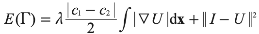
如果用 λ|c1-c2| 替换 ROF 方程 (1.1) 中的 λ,最小化 Chan-Vese 模型现在转变成为设定阈值的 ROF 降噪问题:

import rof
from pylab import *
from PIL import Image
# import scipy.misc
import imageio
from skimage import *

im1 = array(Image.open('../data/flower32_t0.png').convert("L"))
im2 = array(Image.open('../data/ceramic-houses_t0.png').convert("L"))
U1, T1 = rof.denoise(im1, im1, tolerance=0.001)
U2, T2 = rof.denoise(im2, im2, tolerance=0.001)

t1 = 0.8  # flower32_t0 threshold
t2 = 0.4  # ceramic-houses_t0 threshold
seg_im1 = img_as_uint(U1 < t1*U1.max())
seg_im2 = img_as_uint(U2 < t2*U2.max())

fig = figure()
gray()
subplot(231)
axis('off')
imshow(im1)

subplot(232)
axis('off')
imshow(U1)

subplot(233)
axis('off')
imshow(seg_im1)

subplot(234)
axis('off')
imshow(im2)

subplot(235)
axis('off')
imshow(U2)

subplot(236)
axis('off')
imshow(seg_im2)

show()

# scipy.misc.imsave('../images/ch09/flower32_t0_result.pdf', seg_im)
imageio.imsave('../images/ch09/flower32_t0_result.pdf', seg_im1)
imageio.imsave('../images/ch09/ceramic-houses_t0_result.pdf', seg_im2)
# fig.savefig('../images/ch09/flower32_t0_result.pdf', seg_im1)
# fig.savefig('../images/ch09/ceramic-houses_t0_result.pdf', seg_im2)

其中ROF 降噪代码rof.py如下：

from numpy import *


def denoise(im,U_init,tolerance=0.1,tau=0.125,tv_weight=100):
    """ An implementation of the Rudin-Osher-Fatemi (ROF) denoising model
        using the numerical procedure presented in Eq. (11) of A. Chambolle
        (2005). Implemented using periodic boundary conditions.
        
        Input: noisy input image (grayscale), initial guess for U, weight of 
        the TV-regularizing term, steplength, tolerance for the stop criterion
        
        Output: denoised and detextured image, texture residual. """
        
    m,n = im.shape #size of noisy image

    # initialize
    U = U_init
    Px = zeros((m, n)) #x-component to the dual field
    Py = zeros((m, n)) #y-component of the dual field
    error = 1 
    
    while (error > tolerance):
        Uold = U
        
        # gradient of primal variable
        GradUx = roll(U,-1,axis=1)-U # x-component of U's gradient
        GradUy = roll(U,-1,axis=0)-U # y-component of U's gradient
        
        # update the dual varible
        PxNew = Px + (tau/tv_weight)*GradUx # non-normalized update of x-component (dual)
        PyNew = Py + (tau/tv_weight)*GradUy # non-normalized update of y-component (dual)
        NormNew = maximum(1,sqrt(PxNew**2+PyNew**2))
        
        Px = PxNew/NormNew # update of x-component (dual)
        Py = PyNew/NormNew # update of y-component (dual)
        
        # update the primal variable
        RxPx = roll(Px,1,axis=1) # right x-translation of x-component
        RyPy = roll(Py,1,axis=0) # right y-translation of y-component
        
        DivP = (Px-RxPx)+(Py-RyPy) # divergence of the dual field.
        U = im + tv_weight*DivP # update of the primal variable
        
        # update of error
        error = linalg.norm(U-Uold)/sqrt(n*m);
        
    return U,im-U # denoised image and texture residual

两幅难以分割图像的分割结果：

 

4、pixellib库

pixellib库是Python图像分割库，跟第9章联系比较紧密，附在这篇博客后面作为本章内容的延伸。

（1）图像的语义分割和实例分割

在pascalvoc上训练的Xception模型进行语义分割，用mask_cnn_coco模型进行实例分割，代码实现：

##step1.导入pixellib模块
import pixellib
from pixellib.semantic import semantic_segmentation
from pixellib.instance import instance_segmentation
##step2.创建用于执行语义分割的类实例
segment_image = semantic_segmentation()
##step3.调用load_pascalvoc_model()函数加载在Pascal voc上训练的Xception模型
segment_image.load_pascalvoc_model("deeplabv3_xception_tf_dim_ordering_tf_kernels.h5")
##step4.调用segmentAsPascalvoc()函数对图像进行分割
##segment_image.segmentAsPascalvoc("path_to_image", output_image_name = "path_to_output_image")
segment_image.segmentAsPascalvoc("./Images/sample1.jpg", output_image_name = "image_new1.jpg", overlay = True)


segment_image = instance_segmentation()

segment_image.load_model("mask_rcnn_coco.h5")

##segment_image.segmentImage("path_to_image", output_image_name = "output_image_path")

segment_image.segmentImage("./Images/sample2.jpg", output_image_name = "image_new2.jpg", show_bboxes = True)

from pylab import *
from PIL import Image
# 添加中文字体支持
from matplotlib.font_manager import FontProperties
font = FontProperties(fname=r"/System/Library/Fonts/PingFang.ttc", size=14)

figure()
subplot(221)
imshow(array(Image.open("./Images/sample1.jpg")))
title(u'原图1', fontproperties=font)
axis("off")

subplot(222)
imshow(array(Image.open("image_new1.jpg")))
title(u'原图1语义分割图', fontproperties=font)
axis("off")

subplot(223)
imshow(array(Image.open("./Images/sample2.jpg")))
title(u'原图2', fontproperties=font)
axis("off")

subplot(224)
imshow(array(Image.open("image_new2.jpg")))
title(u'原图2实例分割图', fontproperties=font)
axis("off")

show()

运行结果：

（2）图像分割应用——图像换背景

代码实现：

import pixellib
from pixellib.tune_bg import alter_bg
import cv2


change_bg = alter_bg()
change_bg.load_pascalvoc_model("deeplabv3_xception_tf_dim_ordering_tf_kernels.h5")
# change_bg.change_bg_img(f_image_path = "sample.jpg",b_image_path = "background.jpg", output_image_name="new_img.jpg")
output = change_bg.change_bg_img(f_image_path = "./Images/p1.jpg",b_image_path = "./Images/flowers.jpg", output_image_name="flowers_bg.jpg")
cv2.imwrite("img.jpg", output)

change_bg = alter_bg()
change_bg.load_pascalvoc_model("deeplabv3_xception_tf_dim_ordering_tf_kernels.h5")
# change_bg.color_bg("sample.jpg", colors = (0,0,255), output_image_name="colored_bg.jpg")
output = change_bg.color_bg("./Images/p1.jpg", colors = (0,0,255), output_image_name="colored_bg.jpg")
cv2.imwrite("img.jpg", output)

change_bg = alter_bg()
change_bg.load_pascalvoc_model("deeplabv3_xception_tf_dim_ordering_tf_kernels.h5")
# change_bg.gray_bg("sample.jpg",output_image_name="gray_img.jpg")
output = change_bg.gray_bg("./Images/p1.jpg",output_image_name="gray_bg.jpg")
cv2.imwrite("img.jpg", output)

hange_bg = alter_bg()
change_bg.load_pascalvoc_model("deeplabv3_xception_tf_dim_ordering_tf_kernels.h5")
# change_bg.blur_bg("sample2.jpg", low = True, output_image_name="blur_img.jpg")
output = change_bg.blur_bg("./Images/p1.jpg", low = True, output_image_name="blur_bg.jpg")
cv2.imwrite("img.jpg", output)


from pylab import *
from PIL import Image
# 添加中文字体支持
from matplotlib.font_manager import FontProperties
font = FontProperties(fname=r"/System/Library/Fonts/PingFang.ttc", size=14)

figure()
subplot(231)
imshow(array(Image.open("./Images/p1.jpg")))
title(u'original p1', fontproperties=font)
axis("off")

subplot(232)
imshow(array(Image.open("./Images/flowers.jpg")))
title(u'original flowers', fontproperties=font)
axis("off")

subplot(233)
imshow(array(Image.open("flowers_bg.jpg")))
title(u'flowers_bg', fontproperties=font)
axis("off")

subplot(234)
imshow(array(Image.open("colored_bg.jpg")))
title(u'colored_bg', fontproperties=font)
axis("off")

subplot(235)
imshow(array(Image.open("gray_bg.jpg")))
title(u'gray_bg', fontproperties=font)
axis("off")

subplot(236)
imshow(array(Image.open("blur_bg.jpg")))
title(u'blur_bg', fontproperties=font)
axis("off")

show()

运行结果：

（3）图像分割应用——视频换背景

代码实现：

import pixellib
from pixellib.tune_bg import alter_bg
import cv2


change_bg = alter_bg()
change_bg.load_pascalvoc_model("deeplabv3_xception_tf_dim_ordering_tf_kernels.h5")

capture = cv2.VideoCapture(0)
while True:
    ret, frame = capture.read()
    output = change_bg.change_frame_img(frame,b_image_path = "./Images/flowers.jpg")  ###将视频背景换成flowers图片
    # output = change_bg.color_frame(frame, colors = (255, 255, 255)) ###将视频背景换成(255, 255, 255)彩色图片
    # output = change_bg.gray_frame(frame)  ###将视频背景换成灰色图片
    # output = change_bg.blur_frame(frame, extreme = True)###将视频背景换成模糊背景
    cv2.imshow("frame", output)
    if  cv2.waitKey(25) & 0xff == ord('q'):
        break
 

其中change_frame_img函数在pixellib库中没有定义，需要去pixellib库中修改源码tune_bg.py，在源码tune_bg.py中加入change_frame_img函数定义：

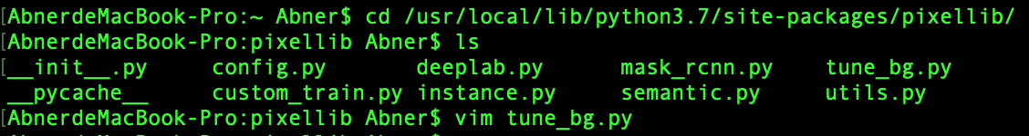
#### ALTER FRAME BACKGROUND WITH A NEW PICTURE ###
def change_frame_img(self, frame, b_image_path, verbose = None):
    if verbose is not None:
      print("processing frame......")

    seg_frame = self.segmentAsPascalvoc(frame, process_frame=True)
    
    bg_img = cv2.imread(b_image_path)
    w, h, _ = frame.shape
    bg_img = cv2.resize(bg_img, (h,w))

    result = np.where(seg_frame[1], frame, bg_img)

    return result

运行结果：

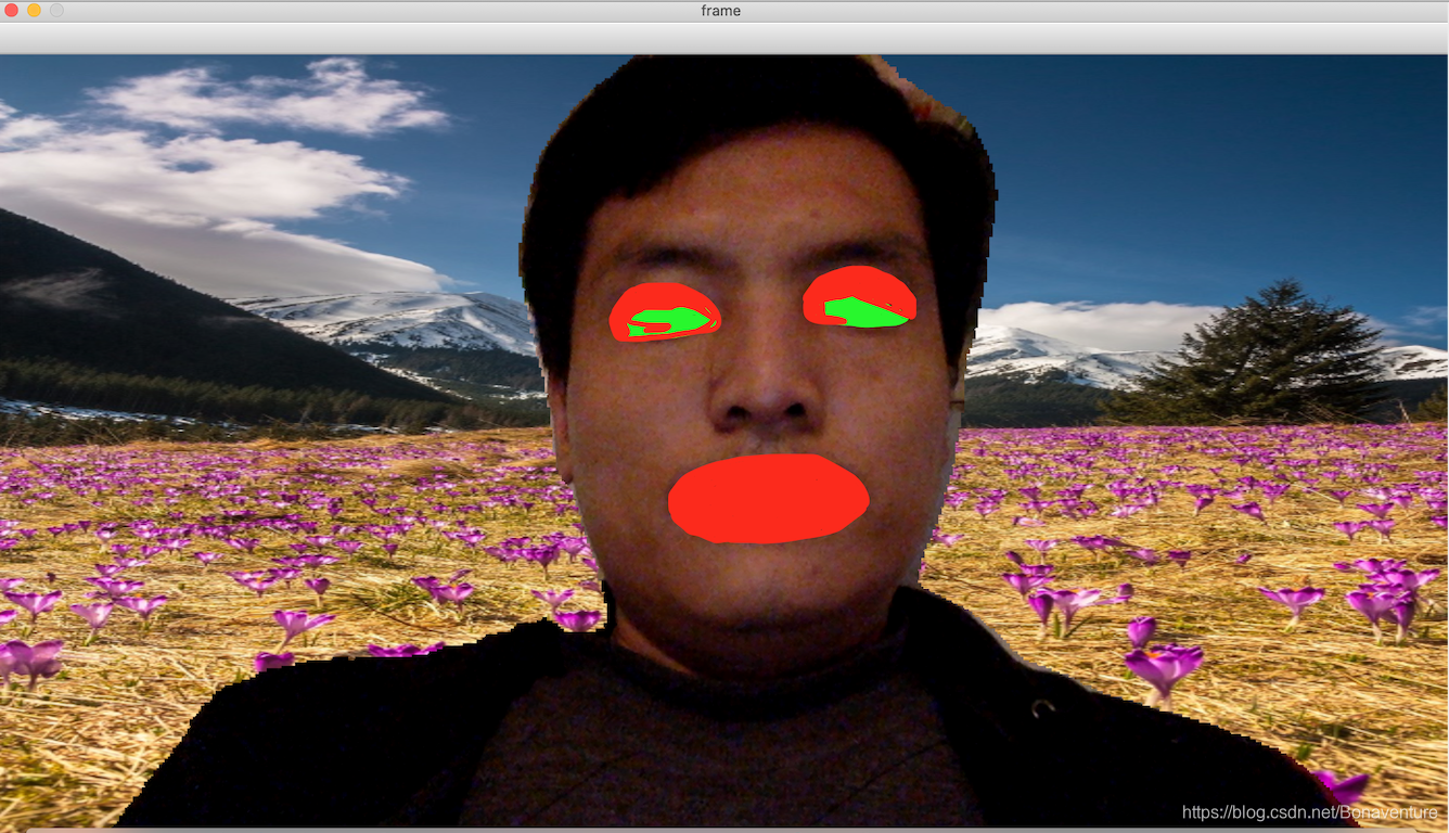
为了保护个人隐私起见，只展示了换flowers背景视频的截图 并涂了涂鸦，其他换彩色、灰色、模糊背景的视频截图就不展示了，感兴趣的可以自行调试代码。

        已经调试过的源码和图片详见：

https://github.com/Abonaventure/pcv-book-code.git

或

https://gitlab.com/Abonaventure/pcv-book-code.git